3 Difference Between PCA and Autoencoder With Python Code

Introduction

 

With more data flooding in the world, extracting out some information or pattern which is the main job of machine learning and deep learning is becoming difficult, the problem is not in algorithms we have made to interpret data but in the data itself, a huge number of dimensions makes it impossible to extract any useful information from the dataset. 

 

Now in order to reduce the dimensions, most machine learning developers use one of the most popular dimensionality reduction techniques, which is nothing else but principal component analysis. But could principle component analysis or T-SNE be the only way to reduce dimensions, or do they always give the desired results?

 

We all must be aware of autoencoders, this deep learning technique is also used by many developers to reduce dimensions, and it sometimes produces even better results than a PCA. 

 

So have you ever been confused about which dimensionality reduction technique to use? This type of problem arises when there is no proper understanding of the working of a dimensionality reduction technique.

 

In this article we are going to compare autoencoders and principal component analysis for a better understanding of which dimensionality reduction technique to use for a specific type of dataset. Let’s begin with understanding principal component analysis first.

 

(Learn more about dimensionality reduction technique as Linear Discriminant Analysis)

 

Principal Component Analysis 

 

Principal component analysis or PCA for short is a dimensionality reduction technique that reduces the lower order dimensions to be very specific. In order to reduce overfitting, the features or dimensions we use must be limited, which also helps in better understanding the relationship between the variables.

---

Analysis of best line

---

With the help of the above image we can understand that in the red line, the errors are huge, therefore this line would produce bad results, whereas in the green line data variables are closely formed above and below the line, therefore this line is best to project and would produce great results.

 

(Also Read: What is adaboost algorithm in ensemble learning)

 

The most important thing to keep in mind while reducing the dimensions is that in order to reduce features, we shall not compromise with the information. In short, the information must not get destroyed in the process, PCA keeps the latter statement in mind and works really well with the reduction of dimensions and information retrieval.

 

Let’s discuss the features of principal component analysis-:

 

1. The main power of the principal component lies in its ability to learn the linear transformation of data.

2. The principal component analysis is exceptionally fast and the computational power is very high which makes it a powerful tool.

3. PCA represents the data information very well in lower dimensions.

4. As the number of features increases, the chances of overfitting of the model decreases significantly.

5. Correlation is vastly removed from the dataset because of the removal of redundant data which makes every principal component different from one another.

6. Due to the fact that most of the features that were not needed by our model get eliminated in the process, the machine learning algorithm performs more efficiently.

 

That was all about the main points about principal component analysis that we needed to know in order to do a fair comparison between PCA and autoencoder.

 

Autoencoder

 

Autoencoder is another dimensionality reduction technique that is majorly used for the regeneration of the input data. Autoencoder is fully capable of not only handling the linear transformation but also the non-linear transformation. 

 

As it is majorly used for the reconstruction of input, the training needs to be as accurate as it could be. The architecture involves an encoder and decoder. 

 

Let’s see the architecture of an autoencoder-:

---

The architecture of a denoising autoencoder

---

The encoders and decoders are neural networks that extract out relevant information from the input and that information is then learned by our model to reconstruct or regenerate the input as it is. Autoencoder uses a backpropagation algorithm to make sure the reduction of errors and accuracy of the model.

 

(Recommended blog: What are autoencoders? How to Implement Convolutional Autoencoder using Keras)

 

Let’s discuss the features of an autoencoder-:

 

1. As we discussed above, the main feature of the autoencoder with the perspective of dimensionality reduction is that it is capable of learning linear as well as non-linear surfaces.

2. With one hidden layer and a sigmoid activation function, it was observed that it performs exactly like principal component analysis.

3. Autoencoder can perform a variety of functions like anomaly detection, information retrieval, image processing, machine translation, and popularity prediction.

4. Autoencoder can give 100% variance of the input data, therefore the regeneration capability for non-linear or curved surfaces is excellent.

 

 

PCA VS Autoencoder

 

With the above introduction and feature analysis of PCA and autoencoders, we are now in the position to do the fair comparison between the both.

 

The first and most obvious point for the comparison is that autoencoder works for both linear and non-linear surfaces, whereas principal component analysis only works for linear surfaces.

---

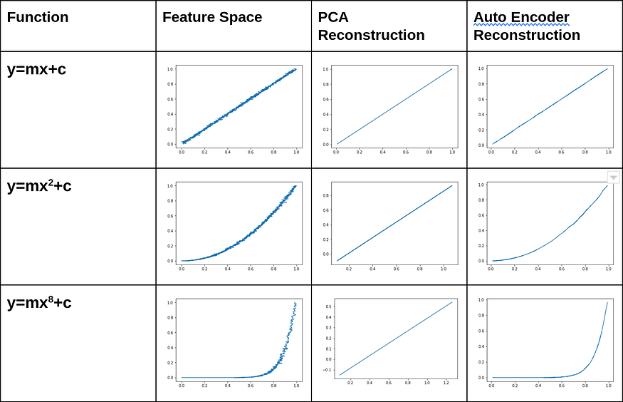
PCA VS Autoencoder on Line Equation,source

---

 

---

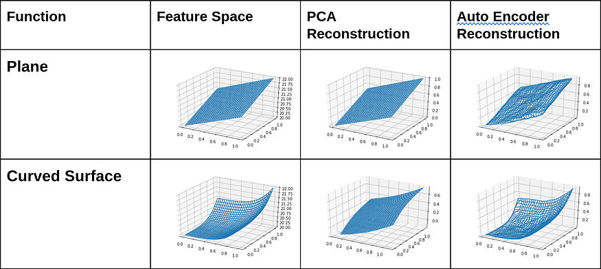
PCA VS Autoencoder on plane and curved surfaces,source

---

The above image shows the reconstruction done by PCA and autoencoders, above are the evidence that proves that PCA is working fine for the straight line equation, might be better than autoencoder in the linear case, but another observation clearly shows it’s inability to map the curved or non-linear surfaces. 

 

The image also perfectly showcases that autoencoders' capability of regenerating the input for both linear and non-linear surfaces with maximum variance is excellent.

 

(Suggested blog: Machine Learning models)

 

This makes one more point clear, that as PCA works for only linear surfaces, we cannot use PCA on the problems where we have to regenerate the non-linear surfaces.

 

1. Computational property

 

As far as computation is concerned, principal component analysis is faster than autoencoder, this might be because an autoencoder uses neural networks which are not computationally cheap.

 

2. Overfitting Analysis

 

Let us understand what is overfitting, when the best fit line is too close to the data points, this closeness leads to the condition where the prediction done by the model on the unseen data goes wrong, therefore the model becomes inaccurate and of no use. Let’s see the below image to visualize overfitting.

---

Visualizing Overfitting condition, source

---

In the above image, we can observe the line a model should get, i.e an ideal line, and the line we get because of overfitting.

 

In between PCA and autoencoder, autoencoders are more prone to get the condition of overfitting of data than PCA, this is because with autoencoder uses backpropagation, that may learn the features to the extent that it works against the idea of the model.

 

3. Similarity between PCA and Autoencoder

 

The autoencoder with only one activation function behaves like principal component analysis(PCA), this was observed with the help of a research and for linear distribution, both behave the same.

 

Implementing PCA is relatively easier than autoencoder due to the fact that there is a python package to implement PCA. Let's see the result of PCA using python.

---

import numpy as np

import matplotlib.pyplot as plt

import pandas as pd

from sklearn.model_selection import train_test_split



from sklearn.decomposition import PCA



dataset = pd.read_csv('../datasets/mnist_data/train.csv')

dataset = dataset.values



X, y = dataset[:, 1:]/255, dataset[:, 0]

X_train, X_test, y_train, y_test = train_test_split(X, y, test_size=0.2)



pca = PCA(n_components=2)

dist = pca.fit_transform(X_train)

dist.shape

(33600, 2)



colors = ['red', 'green', 'blue', 'yellow', 'pink', 'black', 'cyan', 'purple', 'gray', 'magenta']



plt.figure()

for i in range(10000):

    plt.scatter(dist[i,0], dist[i,1], color=colors[y_train[i]])

---

---

In the above code, we have simply imported the PCA package from sklearn. Afterwards we read the dataset with the help of pandas library, splitted the dataset using the train_test_split package that we imported. Lastly, we fit our model on a training dataset and visualize it using the matplotlib library.

 

 

Conclusion

 

PCA and autoencoder are two of the most used dimensionality reduction techniques used by machine learning researchers, therefore, the proper analysis was required on when to use these techniques and when not to. 

 

(Must catch: Machine Learning tools)

 

We have also successfully analysed the weaknesses or the limitations of PCA as well as autoencoders.